Introduction

What is actigraphy? How do we use R?

C. William Yao, Samuel Szocs

What will be covered in this tutorial?

This specific tutorial is designed to give users a gentle introduction to actigraphy and R. For tutorials on how to use ActiGlobe, please go to the rest of the tutorials in this package.

Load the Libraries

library (ActiGlobe)

### Optional Library
# library(zeallot)

If any of the packages have yet to be installed, we can always install them using the function install.packages().

Introduction

What is Actigraphy?

Actigraphy is a non-invasive method used for measuring sleep/wake cycles by using a small device, usually in the form of a wrist-worn watch. It is the easiest way to measure sleep in the field and is widely used in the realm of sleep research due to its extended recording time and ease of use (Smith et al., 2018). An actigraphy device has a built-in accelerometer that measures movement, allowing researchers to objectively track activity patterns over days, weeks, or even months.

Understanding Accelerometers and Gyroscopes

Modern actigraphy devices rely on sophisticated sensors to capture movement data:

Accelerometers

An accelerometer is a sensor that measures acceleration, or more simply, motion in one direction. It works by converting physical movement into electrical signals that the device can interpret and store. A 3-axis (or tri-axial) accelerometer measures acceleration along three perpendicular axes (X, Y, and Z), which correspond to different directions in three-dimensional space. This allows the device to track all types of motion, whether you are walking, running, or lying in bed.

More specifically, an actigraph outputs the magnitude of acceleration (i.e., the vector magnitude of acceleration across all three axes), which is then used by algorithms to classify periods of activity versus rest. For instance, if you are out on a run, as your feet pound against the pavement and your arm swings back and forth, the device on your wrist will detect a sharp increase in the magnitude of acceleration, signaling that you are wide awake and on the move. In contrast, if you are curled up in bed fast asleep, the magnitude will greatly decrease and stabilize, allowing the device to easily discern that you are in a period of sleep or rest.

Gyroscopes

While accelerometers measure linear acceleration, gyroscopes measure angular velocity or rotational movement. Some advanced actigraphy devices incorporate gyroscopes to provide a more complete picture of movement. By combining data from both accelerometers and gyroscopes, these devices can better distinguish between different types of activities (e.g., walking vs. cycling) and reduce errors caused by device orientation.

On-Device Filtering and Data Acquisition

To enable prolonged and uninterrupted data collection while managing storage limitations, most clinical and research-grade actigraphy devices implement on-device filtering and data processing:

Signal Processing

Raw acceleration signals from the accelerometer are typically sampled at high frequencies (e.g., 32 Hz or higher). However, storing raw high-frequency data for weeks or months would require enormous storage capacity. To address this, devices apply on-device signal processing:

1. Bandpass Filtering: Raw acceleration signals are filtered to remove high-frequency noise and low-frequency drift, typically retaining frequencies associated with human movement (approximately 0.25–3 Hz).

2. Magnitude Calculation: The device computes the vector magnitude of acceleration across the three axes:

   \(\text{Magnitude} = \sqrt{x^2 + y^2 + z^2}\)

   where \(x\), \(y\), and \(z\) represent acceleration along each axis.

3. Epoch Aggregation: The filtered magnitude values are aggregated over fixed time intervals called epochs (commonly 15, 30, or 60 seconds). Aggregation methods include summing, averaging, or taking the maximum value within each epoch.

4. Activity Counts: The resulting value for each epoch is stored as an “activity count” — a unitless measure that represents the amount of movement detected during that time period.

This approach dramatically reduces data storage requirements while preserving the essential information needed for sleep/wake analysis and circadian rhythm assessment.

Time Stamping and Time Zone Considerations

To allow for prolonged and uninterrupted data collection, most clinical and research-grade actigraphy devices record only the time and time zone at the initiation of recording. When no travel occurs during the recording period, one can easily infer the time coordinates of all recorded activity counts.

However, time zone changes during data collection present a unique challenge. For example, if a Canadian researcher is initializing devices for a study that collects data before, during, and after travel to Europe, they face a difficult choice: Should the watches be set to Montreal time (UTC-4) or Paris time (UTC+2)? Unfortunately, most actigraphy devices are not flexible enough to automatically adjust for time zone changes during recording.

The Need for ActiGlobe

When a wearer is engaged in long-distance or cross-time-zone travel, the fixed time zone setting becomes problematic. The time zone switch is not automatically recorded or adjusted, which can lead to significant misinterpretation of the data.

Consider the example shown in Figure 1 below from an Actiwatch® device (Varesco et al., 2024). When looking at the raw data without adjustment, the activity count appears noticeably high in the middle of the night (on/right side of the blue line) around November 5th. Moreover, the activity count is low in the middle of the day, leading to the erroneous conclusion that the subject was sleeping during the day and awake at night.

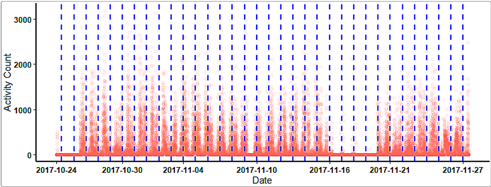
Figure 1: Unadjusted actigraphy data showing apparent day-night reversal due to unaccounted time zone change.

This issue is due to a time zone change that the hardware and software are not aware of. The device continues recording throughout the travel period; thus, the data becomes confusing and produces skewed outcomes. Unaltered data after cross-time-zone travel makes processing and extracting results much more complicated and can lead to incorrect scientific conclusions.

ActiGlobe was developed specifically to address this challenge. By allowing researchers to specify travel logs and time zone transitions, ActiGlobe can adjust actigraphy data to reflect the correct local time throughout the recording period. This ensures that analyses of sleep/wake patterns, circadian rhythms, and activity levels are accurate and interpretable, even when participants travel across multiple time zones.

Figure 2 shows the same data after time zone adjustment using ActiGlobe:

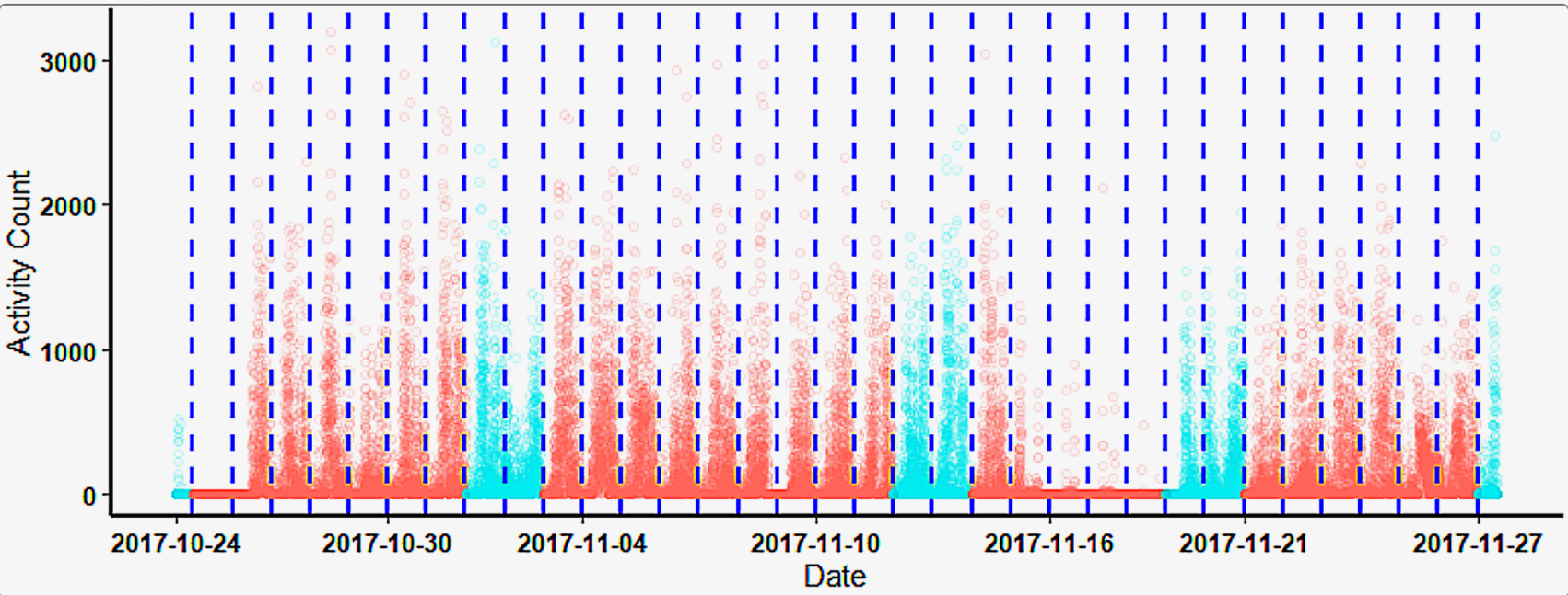
Figure 2: Adjusted actigraphy data showing correct sleep/wake patterns after time zone correction.

After adjustment, the data clearly shows appropriate sleep periods at night and activity during the day, demonstrating the importance of proper time zone handling in actigraphy research.

Getting Started with ActiGlobe

Now that you understand the fundamentals of actigraphy and the challenges of time zone adjustments, you are ready to explore the ActiGlobe package. The following vignettes will guide you through:

• Time-Shift Adjustment: Learn how to adjust actigraphy data for time zone changes and daylight saving time transitions.
• Circadian Analysis: Perform cosinor analysis to characterize circadian rhythms and estimate parameters like MESOR, amplitude, and acrophase.
• Graphic Reports: Generate comprehensive visual reports to communicate your findings effectively.

We encourage you to work through each tutorial to become familiar with the ActiGlobe workflow and discover how this tool can enhance your actigraphy research.

---

Getting Started with R: Essential Skills and Pro Tips

R is a powerful, specialized language for data analysis, statistics, and visualization. Whether you are a new user or an experienced analyst, mastering R’s ecosystem will streamline your workflow—especially when working with packages like ActiGlobe.

Quick Start: Running R

• Install R: Download from CRAN.
• Choose an IDE: RStudio is the gold standard for R, providing an all-in-one interface for scripting, output, packages, and visualization.
  • Alternatives: Visual Studio Code with R extensions, or even Google Colab for running R code via Jupyter interface.

Try out a basic calculation:

2 + 2
#> [1] 4

To reuse the value later, assign it to a variable:

x <- 
  2 + 2

## We can verify it by printing the stored value in x:
print(x)
#> [1] 4

Why R? Robust and Reliable

R’s CRAN committee reviews every package rigorously for compatibility and correctness on all major operating systems. This strict review process in unique among common programming languages (such as Python’s PyPI and MATLAB) in the world of research. In addition, CRAN periodically recheck existing packages compatibility to ensure they continue to meet standards as R evolves. While these checks may introduce some delays in package updates, they provide a crucial layer of quality assurance and avoid version-bounded issues (a common issue among python libraries). For this reason, the primary development of ActiGlobe is and will be in R to ensure long-term stability and reliability for users.

Essential Keyboard Shortcuts (RStudio and General Use)

Speed up coding with these shortcuts (useful in RStudio):

Description	Windows_Linux	MacOS
Autocomplete (TAB)	TAB	TAB
Run line/selection	Ctrl + Enter	Cmd + Enter
Pipe %>%	Ctrl + Shift + M	Cmd + Shift + M
Comment/uncomment	Ctrl + Shift + C	Cmd + Shift + C
Find/replace	Ctrl + F	Cmd + F
Select all	Ctrl + A	Cmd + A
Save script	Ctrl + S	Cmd + S
Insert new code chunk	Ctrl + Alt + I	Cmd + Option + I
Go to file/function	Ctrl + .	Cmd + .
Show documentation	F1	F1

Reference: RStudio Keyboard Shortcuts

< Pro-tip > Autocomplete (TAB) works for functions, arguments, and file names—use it to boost accuracy and speed.

Basic Programming & Package Management

R is built for clarity:

# Assign a value
x <- 42

# Create a vector
numbers <- c (1, 2, 3, 4, 5)

mean (numbers)

Install and load a package:

install.packages ("dplyr")
library (dplyr)

Install multiple packages at once:

install.packages (c ("dplyr", "tidyr", "ggplot2"))

See this R-bloggers intro guide for practical examples and tips.

Fundamental Packages & Functions

• Base R: mean(), sd(), summary(), plot(), hist()
• Core Packages:
  • stats: Statistical modeling and classic tests.
  • dplyr: Data wrangling (select, filter, mutate, group, summarize).
  • tidyr: Data tidying (pivot_longer, pivot_wider, separate, unite).
  • ggplot2: Elegant data visualization.

Example: Filter and Plot with dplyr & ggplot2

## Import libraries
library (dplyr)
library (ggplot2)
library (tidyr)

## Create sample data
df <- tibble (ID = 1:6, value = c(10, 15, 18, 12, 11, 17))

## Filter values greater than 12 and plot
df %>%
  filter (value > 12) %>%
  ggplot (aes (x = ID, y = value)) +
  geom_col ()

### Data Wrangling, Visualization, and Reproducibility Tutorials

• Data Wrangling with dplyr
• Data Visualization with ggplot2
• Reproducible Analyses with RMarkdown

Avoiding Package Duplication: Managing .libPaths()

To avoid duplicate installations and manage shared settings across operating systems, we recommend users to customize .libPaths():

# Display current library locations
.libPaths ()

# Set a custom/shared R library (adjust for OS)
.libPaths ("C:/R/libraries")    # Windows (Out of the `Program Files` folder)
.libPaths ("~/R/libraries")     # Linux/MacOS

To permanently set this path, add the above line to your Rprofile.site file:

• Windows:
  C:/Program Files/R/R-x.y.z/etc/Rprofile.site

• Linux/MacOS:
  /usr/lib/R/etc/Rprofile.site

Advanced-setting: Users with multiple PCs may consider storing libraries on a synced drive (Dropbox, OneDrive) when switching between computers. This will also require modifying the Rprofile.site location.

Try install directly to the new path:

# Verify the new library path. The new path should be the first.
print (.liibPaths())

install.packages ("lubridate")

Common Pitfalls and Best Practices

• Error Handling:
  Use tryCatch() to manage unexpected errors and keep analyses running.

tryCatch (log ("a"), error = function (e) "Not a number")

• Reproducibility:
  Use RMarkdown (.Rmd) to combine code, results, and documentation.
  Run knitr::knit("myreport.Rmd") to generate reproducible reports.

• Efficient Code:

  • Use vectorized functions: Replace for loops with apply or vectorized alternatives when possible.
  • Avoid using attach() to prevent hidden bugs in scope.

• Debugging:

  • Use browser(), traceback(), or RStudio’s built-in debugger.
  • Check the RStudio Troubleshooting FAQ for solutions to common issues.

• Learning from the Community:
  Ask questions or find solutions on R-bloggers and Stack Overflow.

Interactive Learning

Besides practice coding locally, we also recommend visiting interactive learning platforms such as:

• DataCamp

• Coursera

Disclaimer: No, we are not sponsored by any of these platforms! We recommend them purely based on their content quality and user experience.

References

Smith, Michael T., et al. “Use of Actigraphy for the Evaluation of Sleep Disorders and Circadian Rhythm Sleep-Wake Disorders: An American Academy of Sleep Medicine Systematic Review, Meta-Analysis, and GRADE Assessment.” Journal of Clinical Sleep Medicine, vol. 14, no. 07, July 2018, pp. 1209–30. DOI: https://doi.org/10.5664/jcsm.7228.

Varesco, G., Yao, C. W., Dubé, E., Simonelli, G., & Bieuzen, F. (2024). “Time zone transitions and actigraphy data adjustment for circadian rhythm research.” The Journal of Physiology. DOI: https://doi.org/10.1113/ep092195.