Circadian-Analysis

What will be covered in this tutorial? This specific tutorial is designed to show users how to use ActiGlobe to perform circadian analysis via cosinor models or Gaussian kernel density estimation (KDE). For data pre-processing or generation of graphic/excel report of daily actigraphy measures, please go to tutorials titled: Time-Shift and Graphic-Report.

Cosinor Analysis

After we segmented the data by date, we can now model the circadian rhythm using the activity scores. For this, we will use the pre-travel recording on the 27^th of October. Since the recording was not affected by the time change. We can simply store the unaffected segments in a new variable called df, which stands for data frame.

# Import data
data ("FlyEast")

BdfList <-
    BriefSum (
        df = FlyEast,
        SR = 1 / 60,
        Start = "2017-10-24 13:45:00",
        TZ = "America/New_York"
    )


# Let's extract actigraphy data from a single day
df <- BdfList$df
df <- subset (df, df$Date == "2017-10-27")

Single-phase Model (i.e., single phase circadian rhythm)

Traditional Cosinor Model fitted via Ordinary Least Sqaure (OLS)

fit.ols <-
    CosinorM (
        time = df$Time,
        activity = df$Activity,
        tau = 24,
        method = "OLS"
    )

### Look at the parameters
fit.ols$coef.cosinor
#>        MESOR Amplitude.24 Acrophase.24      Beta.24     Gamma.24 
#>   177.297222   161.296243    -2.896002  -156.456357   -39.215893

### Plot
ggCosinorM (fit.ols)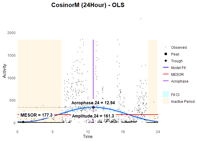

Figure 1: Fitting of OLS-based Cosinor Model

Note

If we process FlyEast using the cosinor::cosinor.lm, we will notice that the results look a bit different. This is because ActiGlobe treats the first time point of the day as 00:00:00, whereas this is sometimes treated as 00:00:00 plus one unit of the device sampling rate due to the use of the sequence generator.

Econometry-modified Cosinor Model with Feasible General Least Square (FGLS)

Besides, the traditional OLS-based cosinor model,CosinorM also allows users to estimate the model using the FGLS-based method. In ActiGlobe, the FGLS was implemented via a weighted residual least square approximation. This two-step process often produces a better representation of the “border” between sleep and wakefulness than traditional OLS. Nevertheless, neither method can realistically capture our activity patterns, given that they are simply single-phase cosinor models.

fit.fgls <-
    CosinorM (
        time = df$Time,
        activity = df$Activity,
        tau = 24,
        method = "FGLS"
    )

### Look at the parameters
fit.fgls$coef.cosinor
#>        MESOR Amplitude.24 Acrophase.24      Beta.24     Gamma.24 
#>   181.169023   183.040124    -2.409542  -136.146165  -122.343405

### Plot
ggCosinorM (fit.fgls)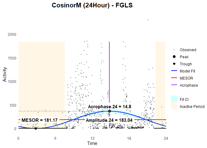

Figure 2: Fitting of FGLS-based Cosinor Model

Dual-phase Model (i.e., 12 + 24hour rhythms)

While certain circadian measures, such as melatonin, often follow a roughly 24-hour single-phase, human activity pattern is generally fragmented. To capture the non-linearity in our activity pattern, it is possible to add more phase components when using CosinorM. Here, we provided two examples of cosinor models with two phase components, each fitted using OLS or FGLS-based methods.

Traditional Cosinor Model fitted via Ordinary Least Sqaure (OLS)

fit.ols2 <-
    CosinorM (
        time = df$Time,
        activity = df$Activity,
        tau = c (12, 24),
        method = "OLS"
    )


fit.ols2$coef.cosinor
#>        MESOR Amplitude.12 Amplitude.24 Acrophase.12 Acrophase.24      Beta.12 
#>  177.2972222  136.4395529  161.2962432   -0.9644981   -2.8960017   77.7472728 
#>      Beta.24     Gamma.12     Gamma.24 
#> -156.4563575 -112.1209756  -39.2158930
fit.ols2$post.hoc
#>           MESOR.ph Bathyphase.ph.time          Trough.ph  Acrophase.ph.time 
#>         182.629625           3.466667         -77.533671          10.783333 
#>            Peak.ph       Amplitude.ph 
#>         442.792922         260.163297


### Plot
ggCosinorM (fit.ols2)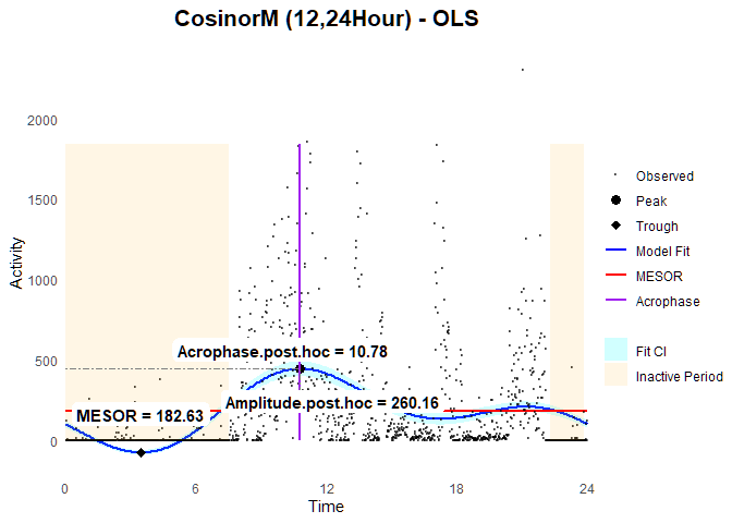

Figure 3: Fitting of the Dual-phase OLS-based Multi-comopnent Cosinor Model

Eocnometry-modified Cosinor Model with Feasible General Least Square (FGLS)

fit.fgls2 <-
    CosinorM (
        time = df$Time,
        activity = df$Activity,
        tau = c (12, 24),
        method = "FGLS"
    )


fit.fgls2$coef.cosinor
#>        MESOR Amplitude.12 Amplitude.24 Acrophase.12 Acrophase.24      Beta.12 
#>  148.6450319   52.7954160  128.4419382   -0.7394464   -2.7311777   39.0074572 
#>      Beta.24     Gamma.12     Gamma.24 
#> -117.7755191  -35.5777211  -51.2470351
fit.fgls2$post.hoc
#>           MESOR.ph Bathyphase.ph.time          Trough.ph  Acrophase.ph.time 
#>         148.959604           3.450000          -8.218935          11.750000 
#>            Peak.ph       Amplitude.ph 
#>         306.138144         157.178540

### Plot
ggCosinorM (fit.fgls2)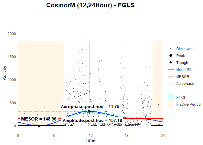

Figure 4: Fitting of the Dual-phase FGLS-based Multi-comopnent Cosinor Model

It is worth noting that we cannot individually interpret each cosinor parameter alone when fitting a multicomponent model. This is because the rest-activity patterns estimated by general linear regression are the cumulative sums of all the fitted cosinor components (i.e., both 12- and 24-hour waves). As such, it is better to use the post hoc-extracted parameters for analysis.

#>    Beta.12   Gamma.12     phi.12 
#>   77.74727 -112.12098   10.15794 
#>    Beta.24   Gamma.24     phi.24 
#> -156.45636  -39.21589   12.93809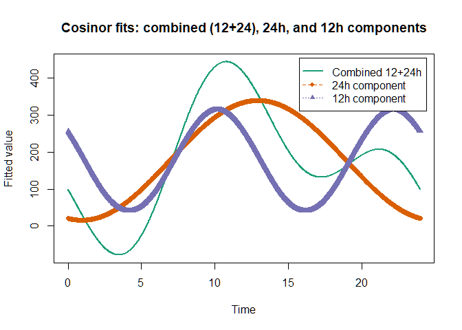

Figure 5 Opening the Dual-phase OLS-based Cosinor Model into 12 and 24hour components

Gaussian Kernel Density Estimation on Circularized Time

Besides the traditional cosinor rhythmetry, ActiGlobe also offers Gaussian kernel density estimation (KDE). In contrast to the traditional cosinor method, CosinrM.KDE uses nonparametric kernel smoothing to map the activity pattern on a circularized time domain. This strategy allows it to better respect the intensity and the duration of the underlying rest-activity patterns, without forcing a sinusoidal shape. To ease transition from cosinor model, we designed CosinorM.KDE to generate cosinor-like parameters by projecting the model onto an imaginary cosinor plane.

fit.KDE <-
    CosinorM.KDE (
        time = df$Time,
        activity = df$Activity
    )

### Look at the parameters
fit.KDE$coef.cosinor
#>        MESOR Amplitude.24 Acrophase.24      Beta.24     Gamma.24 
#>   177.327801   157.744980    -2.895821  -153.004740   -38.380048
fit.KDE$post.hoc
#>           MESOR.ph Bathyphase.ph.time          Trough.ph  Acrophase.ph.time 
#>         296.160217           5.433333           9.099325          10.483333 
#>            Peak.ph       Amplitude.ph 
#>         583.221110         287.060893

ggCosinorM (fit.KDE)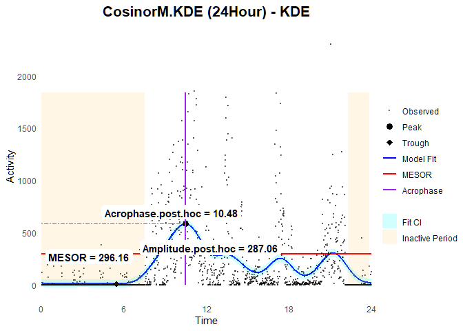

Figure 6: Fitting of Circularized Gaussian Kernel Density Estimation

It is worth noting that while CosinorM.KDE does provide a variance and standard error for the fitted rest-activity pattern; this is a density‑based signal‑processing strategy, not a regression model. As a signal‑processing technique, CosinorM.KDE lacks the ability to directly provide standard errors or confidence intervals for cosinor parameters and related post hoc estimates (e.g., bathyphase). Thankfully, we can use bootstrap resampling to empirically estimate confidence intervals and standard errors for these post‑hoc parameters. Note that CosinorM.KDE is designed to stabilize estimates when data are irregularly spaced or limited to short recording intervals.

boot.seci (
    object = fit.KDE,
    ci_level = 0.95,
    n = 100
) ### for demonstration, the number of bootstraps was limited to 100.
#>                    Estimate Std Error t value    2.5%   97.5%
#> MESOR                177.30      4.60   38.56  168.99  185.45
#> Amplitude.24         157.54      7.15   22.06  145.39  171.51
#> Acrophase.24          -2.89      0.04  -73.15   -2.96   -2.82
#> Beta.24             -152.35      7.90  -19.38 -167.59 -138.84
#> Gamma.24             -39.61      5.28   -7.27  -48.31  -29.42
#> MESOR.ph             295.55     14.50   20.43  266.18  324.46
#> Bathyphase.ph.time     4.35      1.83    2.96    0.60    6.13
#> Trough.ph              8.12      1.84    4.93    5.09   11.66
#> Acrophase.ph.time     10.50      0.31   33.60    9.97   11.05
#> Peak.ph              582.97     29.10   20.04  522.64  638.85
#> Amplitude.ph         287.43     14.66   19.58  257.36  314.75

Currently, was designed to compute standard errors and confidence intervals in serial processes, which means that it will take some time to finish the computation.

Visualized Model Comparisons

### For external graphic plot.
library (ggplot2)

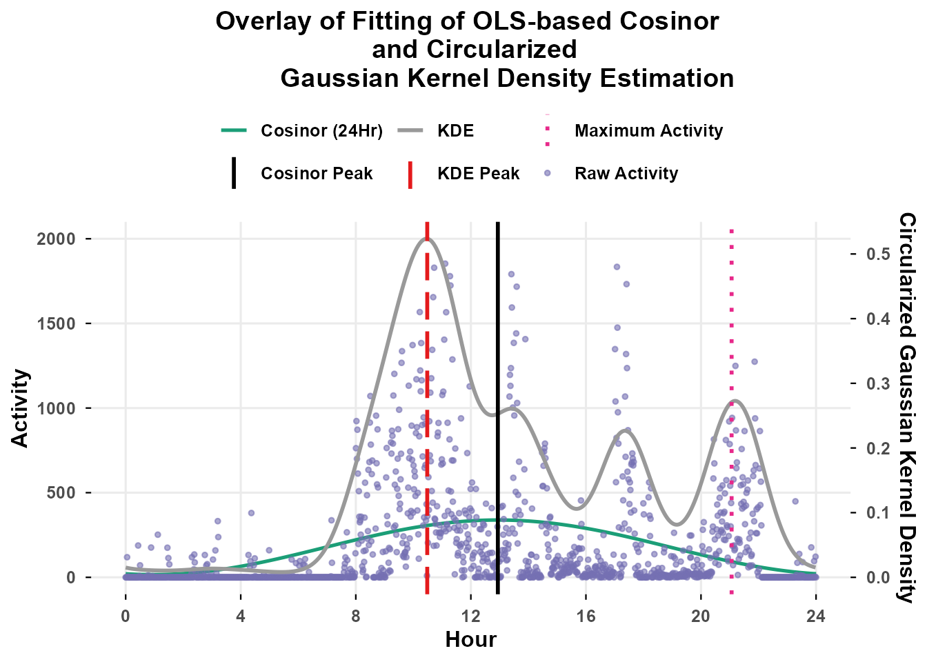
OLS-Cosinor vs. Kernel Density Estimation

When we compare the KDE-based estimate with the OLS-based cosinor model, we can immediately see that CosinorM.KDE better captures the complexity of the wearer’s activity pattern. Since CosinorM.KDE does not assume a specific pattern of activity, it avoids introducing bias from assumptions or model specifications into the rest-activity-based circadian parameters. Figure 7: Overlay of Fitting of OLS-based Cosinor and Circularized Gaussian Kernel Density Estimation

Cosinor Analysis and Circularized Kernel Density Estimation

C. William Yao

Cosinor Analysis

Single-phase Model (i.e., single phase circadian rhythm)

Traditional Cosinor Model fitted via Ordinary Least Sqaure (OLS)

Note

Econometry-modified Cosinor Model with Feasible General Least Square (FGLS)

Dual-phase Model (i.e., 12 + 24hour rhythms)

Traditional Cosinor Model fitted via Ordinary Least Sqaure (OLS)

Eocnometry-modified Cosinor Model with Feasible General Least Square (FGLS)

Gaussian Kernel Density Estimation on Circularized Time

Visualized Model Comparisons

OLS-Cosinor vs. Kernel Density Estimation